Ben Pitler
Human rights defender and University of Washington MBA candidate, data science/analytics track. Passionate about using data science to achieve justice.
This portfolio details my use of data science to investigate and document violations of international human rights law. Please direct all questions and requests to collaborate to ds4hrbp@protonmail.com
LinkedIn
Using fmsb radarchart to visualize preliminary death sentences in Egypt (2011-2018) and executions in Saudi Arabia (2014-2019)
Radar charts of preliminary death sentences in Egypt by month
Here, I used the radarchart function from the fmsb package to create radar charts (also known as spider charts) to track preliminary death sentences handed down by Egyptian courts in each year between 2011 and 2018. (see here for more information about my data work in Egypt). There is some controversy around the use of radar charts–some people rightly point out that this is a flawed type of visualization, given its tendency to overemphasize large outlier values, obscure smaller values, and group categories into meaningless orders. That said, I think these charts are quite useful for this specific purpose, as I am tracking data by an ordinal month variable, and also because the point here is to get an idea of how death sentences trended over time, not necessarily to grasp exact numbers. Also, radar charts look cool.
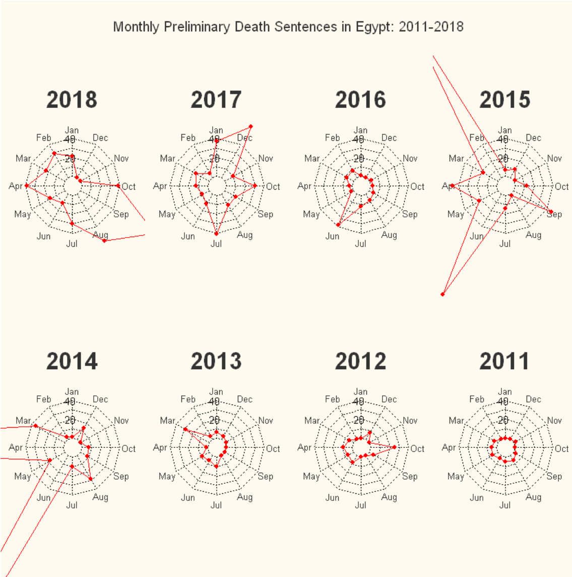
The axes here range from 0 to 40, and we see that from 2011 to mid-2013, when el-Sisi came to power, preliminary death sentences remained relatively muted; courts in Egypt sentenced 30 or more people to death in one month only one time. However, after el-Sisi came to power, preliminary death sentences increased drastically, with courts routinely sentencing 40 or more people to death in a single month. The charts are imperfect in that the values extend well past the axis limits in several instances, making it difficult to ascertain how many people were sentenced to death in those months (although I like the look of that, aesthetically speaking), but I think they do a good job of communicating the overall trend: death sentences in Egypt are way, way up.
The code for this viz looks like this:
library(fmsb)

[//]: # Reading in the data from .csv file. This .csv contains 3000+ rows, each of which contains information on a discrete individual sentenced to death by an Egyptian court between 2011 and 2018
EDPI <- read.csv ("egypt_individuals_csv.csv", header=TRUE, sep=",", stringsAsFactors=FALSE)

[//]: # Converting the column containing the date of each death sentence to date type
EDPI$Crim.1.Judgement.Date <- as.Date (EDPI$Crim.1.Judgement.Date, "%m/%d/%Y")

[//]: # Creating a new column by extracting the month of each sentence
EDPI$Crim.1.Judgement.Month <- format(EDPI$Crim.1.Judgement.Date, "%m")

[//]: # Converting month of sentence column to numeric so the for loop below doesn't exclude months 01-09
EDPI$Crim.1.Judgement.Month <- as.numeric(EDPI$Crim.1.Judgement.Month)

[//]: # Creating eight empty lists of 12 NULL values, to be filled by the for loop
egypt_years_list_2011 <- vector("list", 12)
egypt_years_list_2012 <- vector("list", 12)
egypt_years_list_2013 <- vector("list", 12)
egypt_years_list_2014 <- vector("list", 12)
egypt_years_list_2015 <- vector("list", 12)
egypt_years_list_2016 <- vector("list", 12)
egypt_years_list_2017 <- vector("list", 12)
egypt_years_list_2018 <- vector("list", 12)

[//]: # for loop that fills each slot of the empty lists with the length of the date column (i.e. number of death sentences) for each month
for (i in 1:12) {
    egypt_years_list_2011[[i]] <- length((subset(EDPI,
        EDPI$Crim.1.Judgement.Month == i & EDPI$Crim.1.Judgement.Year == 2011))$Crim.1.Judgement.Year)

    egypt_years_list_2012[[i]] <- length((subset(EDPI,
        EDPI$Crim.1.Judgement.Month == i & EDPI$Crim.1.Judgement.Year == 2012))$Crim.1.Judgement.Year)

    egypt_years_list_2013[[i]] <- length((subset(EDPI,
        EDPI$Crim.1.Judgement.Month == i & EDPI$Crim.1.Judgement.Year == 2013))$Crim.1.Judgement.Year)

    egypt_years_list_2014[[i]] <- length((subset(EDPI,
        EDPI$Crim.1.Judgement.Month == i & EDPI$Crim.1.Judgement.Year == 2014))$Crim.1.Judgement.Year)

    egypt_years_list_2015[[i]] <- length((subset(EDPI,
        EDPI$Crim.1.Judgement.Month == i & EDPI$Crim.1.Judgement.Year == 2015))$Crim.1.Judgement.Year)

    egypt_years_list_2016[[i]] <- length((subset(EDPI,
        EDPI$Crim.1.Judgement.Month == i & EDPI$Crim.1.Judgement.Year == 2016))$Crim.1.Judgement.Year)

    egypt_years_list_2017[[i]] <- length((subset(EDPI,
        EDPI$Crim.1.Judgement.Month == i & EDPI$Crim.1.Judgement.Year == 2017))$Crim.1.Judgement.Year)

    egypt_years_list_2018[[i]] <- length((subset(EDPI,
        EDPI$Crim.1.Judgement.Month == i & EDPI$Crim.1.Judgement.Year == 2018))$Crim.1.Judgement.Year)
}

[//]: # Turning each list into a dataframe
egypt_2011_prelim <- data.frame(egypt_years_list_2011)
egypt_2012_prelim <- data.frame(egypt_years_list_2012)
egypt_2013_prelim <- data.frame(egypt_years_list_2013)
egypt_2014_prelim <- data.frame(egypt_years_list_2014)
egypt_2015_prelim <- data.frame(egypt_years_list_2015)
egypt_2016_prelim <- data.frame(egypt_years_list_2016)
egypt_2017_prelim <- data.frame(egypt_years_list_2017)
egypt_2018_prelim <- data.frame(egypt_years_list_2018)

[//]: # Renaming the dataframe columns
colnames (egypt_2011_prelim) <- c ("Jan", "Feb", "Mar", "Apr", "May", "Jun", "Jul", "Aug", "Sep", "Oct", "Nov", "Dec")
colnames (egypt_2012_prelim) <- c ("Jan", "Feb", "Mar", "Apr", "May", "Jun", "Jul", "Aug", "Sep", "Oct", "Nov", "Dec")
colnames (egypt_2013_prelim) <- c ("Jan", "Feb", "Mar", "Apr", "May", "Jun", "Jul", "Aug", "Sep", "Oct", "Nov", "Dec")
colnames (egypt_2014_prelim) <- c ("Jan", "Feb", "Mar", "Apr", "May", "Jun", "Jul", "Aug", "Sep", "Oct", "Nov", "Dec")
colnames (egypt_2015_prelim) <- c ("Jan", "Feb", "Mar", "Apr", "May", "Jun", "Jul", "Aug", "Sep", "Oct", "Nov", "Dec")
colnames (egypt_2016_prelim) <- c ("Jan", "Feb", "Mar", "Apr", "May", "Jun", "Jul", "Aug", "Sep", "Oct", "Nov", "Dec")
colnames (egypt_2017_prelim) <- c ("Jan", "Feb", "Mar", "Apr", "May", "Jun", "Jul", "Aug", "Sep", "Oct", "Nov", "Dec")
colnames (egypt_2018_prelim) <- c ("Jan", "Feb", "Mar", "Apr", "May", "Jun", "Jul", "Aug", "Sep", "Oct", "Nov", "Dec")

[//]: # Combining all the dataframe rows into one dataframe
egypt_final <- rbind(egypt_2011_prelim, egypt_2012_prelim, egypt_2013_prelim, egypt_2014_prelim, egypt_2015_prelim, egypt_2016_prelim, egypt_2017_prelim, egypt_2018_prelim)

[//]: # Renaming the new dataframe rows
rownames (egypt_final) <- c(2011,2012,2013, 2014, 2015, 2016, 2017, 2018)

[//]: # To use radarchart(), the df has to have max and min values in each column. The below adds max and min rows of 0 and 40, each repeating 12 times
egypt_final <- rbind(egypt_final, (rep.int(40, 12)))
egypt_final <- rbind(egypt_final, (rep.int(0, 12)))

[//]: # Rearranging the rows because the pattern of rows for radarchart() to work has to be max, min, data:
egypt_final <- egypt_final[c(9,10,8,7,6,5,4,3,2,1),]

[//]: # Making the chart matrix

par(xpd=TRUE, mar=c(1, 1, 1, 1), #xpd prevents labels from being cut off. mar decreases default margin.
   oma=c(0,0,5,0),
   bg = "floralwhite",
   cex = 1,
   col="gray20"
   )
layout(matrix(1:8, ncol=4))

radarchart(egypt_final[c(1,2,3),],
          axistype=1,
           caxislabels=c("","",20,"",40),
          calcex=1.1,
          axislabcol="black",
           cglcol="black",
           pcol=2)
mtext(side = 3, line = -4, at = 0, cex = 1.75, "2018", font = 2)

radarchart(egypt_final[c(1,2,7),],
           axistype=1,
           caxislabels=c("","",20,"",40),
          calcex=1.1,
          axislabcol="black",
           cglcol="black",
           pcol=2)
mtext(side = 3, line = -4, at = 0, cex = 1.75, "2014", font = 2)

radarchart(egypt_final[c(1,2,4),],
           axistype=1,
           caxislabels=c("","",20,"",40),
          calcex=1.1,
          axislabcol="black",
           cglcol="black",
           pcol=2)
mtext(side = 3, line = -4, at = 0, cex = 1.75, "2017", font = 2)

radarchart(egypt_final[c(1,2,8),],
           axistype=1,
           caxislabels=c("","",20,"",40),
          calcex=1.1,
          axislabcol="black",
           cglcol="black",
           pcol=2)
mtext(side = 3, line = -4, at = 0, cex = 1.75, "2013", font = 2)

radarchart(egypt_final[c(1,2,5),],
           axistype=1,
           caxislabels=c("","",20,"",40),
          calcex=1.1,
          axislabcol="black",
           cglcol="black",
           pcol=2)
mtext(side = 3, line = -4, at = 0, cex = 1.75, "2016", font = 2)

radarchart(egypt_final[c(1,2,9),],
           axistype=1,
           caxislabels=c("","",20,"",40),
          calcex=1.1,
          axislabcol="black",
           cglcol="black",
           pcol=2)
mtext(side = 3, line = -4, at = 0, cex = 1.75, "2012", font = 2)

radarchart(egypt_final[c(1,2,6),],
           axistype=1,
           caxislabels=c("","",20,"",40),
          calcex=1.1,
          axislabcol="black",
           cglcol="black",
           pcol=2)
mtext(side = 3, line = -4, at = 0, cex = 1.75, "2015", font = 2)

radarchart(egypt_final[c(1,2,10),],
           axistype=1,
           caxislabels=c("","",20,"",40),
          calcex=1.1,
          axislabcol="black",
           cglcol="black",
           pcol=2)
mtext(side = 3, line = -4, at = 0, cex = 1.75, "2011", font = 2)

mtext("Monthly Preliminary Death Sentences in Egypt: 2011-2018", side = 3, line = 2, outer = TRUE)
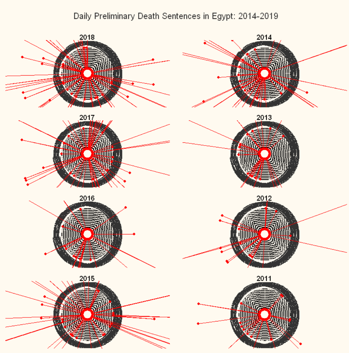
Radar charts of preliminary death sentences in Egypt by day
Below is another version of a radar chart tracking the same data, but here we are tracking death sentences by day, rather than by month. These I will admit are perhaps not the most useful from an insights perspective, I just like the way they look. That said, because the outer limit of the axes on these charts is 1, the charts show you which periods of which years had zero death sentences, which had one death sentence, and which had more than one death sentence. As such, we can see the extent to which death sentences were evenly distributed throughout a given year, and where there were gaps.
The code for this viz looks like this:
library(fmsb)

[//]: # Reading in the Egypt data
EDPI <- read.csv ("egypt_individuals_csv.csv", header=TRUE, sep=",")

[//]: # Converting the column containing the date of each death sentence to date type
EDPI$Crim.1.Judgement.Date <- as.Date (EDPI$Crim.1.Judgement.Date, "%m/%d/%Y")

[//]: # Creating year of death sentence and day of year of death sentence columns
EDPI$Crim.1.Judgement.Day.of.Year <- format(EDPI$Crim.1.Judgement.Date, "%j")
EDPI$Crim.1.Judgement.Year <- format(EDPI$Crim.1.Judgement.Date, "%Y")

[//]: # Converting year and day of year columns to numeric
EDPI$Crim.1.Judgement.Year <- as.numeric(EDPI$Crim.1.Judgement.Year)
EDPI$Crim.1.Judgement.Day.of.Year <- as.numeric(EDPI$Crim.1.Judgement.Day.of.Year)

[//]: # Creating eight empty lists of 365 NULL Values
egypt_daily_2011_list <- vector("list", 365)
egypt_daily_2012_list <- vector("list", 365)
egypt_daily_2013_list <- vector("list", 365)
egypt_daily_2014_list <- vector("list", 365)
egypt_daily_2015_list <- vector("list", 365)
egypt_daily_2016_list <- vector("list", 365)
egypt_daily_2017_list <- vector("list", 365)
egypt_daily_2018_list <- vector("list", 365)


[//]: # for loop that fills each slot of the empty lists with the length of the day of year column (i.e. number of death sentences) for each month

for (i in 1:365) {
    egypt_daily_2011_list[[i]] <- length((subset(EDPI,
        EDPI$Crim.1.Judgement.Day.of.Year == i & EDPI$Crim.1.Judgement.Year == 2011))$Crim.1.Judgement.Day.of.Year)

    egypt_daily_2012_list[[i]] <- length((subset(EDPI,
        EDPI$Crim.1.Judgement.Day.of.Year == i & EDPI$Crim.1.Judgement.Year == 2012))$Crim.1.Judgement.Day.of.Year)

    egypt_daily_2013_list[[i]] <- length((subset(EDPI,
        EDPI$Crim.1.Judgement.Day.of.Year == i & EDPI$Crim.1.Judgement.Year == 2013))$Crim.1.Judgement.Day.of.Year)

    egypt_daily_2014_list[[i]] <- length((subset(EDPI,
        EDPI$Crim.1.Judgement.Day.of.Year == i & EDPI$Crim.1.Judgement.Year == 2014))$Crim.1.Judgement.Day.of.Year)

    egypt_daily_2015_list[[i]] <- length((subset(EDPI,
        EDPI$Crim.1.Judgement.Day.of.Year == i & EDPI$Crim.1.Judgement.Year == 2015))$Crim.1.Judgement.Day.of.Year)

    egypt_daily_2016_list[[i]] <- length((subset(EDPI,
        EDPI$Crim.1.Judgement.Day.of.Year == i & EDPI$Crim.1.Judgement.Year == 2016))$Crim.1.Judgement.Day.of.Year)

    egypt_daily_2017_list[[i]] <- length((subset(EDPI,
        EDPI$Crim.1.Judgement.Day.of.Year == i & EDPI$Crim.1.Judgement.Year == 2017))$Crim.1.Judgement.Day.of.Year)

    egypt_daily_2018_list[[i]] <- length((subset(EDPI,
        EDPI$Crim.1.Judgement.Day.of.Year == i & EDPI$Crim.1.Judgement.Year == 2018))$Crim.1.Judgement.Day.of.Year)
    }

[//]: # Turning each list into a dataframe
egypt_2011_daily_df <- data.frame(egypt_daily_2011_list)
egypt_2012_daily_df <- data.frame(egypt_daily_2012_list)
egypt_2013_daily_df <- data.frame(egypt_daily_2013_list)
egypt_2014_daily_df <- data.frame(egypt_daily_2014_list)
egypt_2015_daily_df <- data.frame(egypt_daily_2015_list)
egypt_2016_daily_df <- data.frame(egypt_daily_2016_list)
egypt_2017_daily_df <- data.frame(egypt_daily_2017_list)
egypt_2018_daily_df <- data.frame(egypt_daily_2018_list)

[//]: # Renaming the dataframe columns
colnames (egypt_2011_daily_df) <- c(1:365)
colnames (egypt_2012_daily_df) <- c(1:365)
colnames (egypt_2013_daily_df) <- c(1:365)
colnames (egypt_2014_daily_df) <- c(1:365)
colnames (egypt_2015_daily_df) <- c(1:365)
colnames (egypt_2016_daily_df) <- c(1:365)
colnames (egypt_2017_daily_df) <- c(1:365)
colnames (egypt_2018_daily_df) <- c(1:365)


[//]: # Combining all the dataframe rows into one dataframe
egypt_daily_final <- rbind(egypt_2011_daily_df, egypt_2012_daily_df, egypt_2013_daily_df, egypt_2014_daily_df, egypt_2015_daily_df, egypt_2016_daily_df, egypt_2017_daily_df, egypt_2018_daily_df)

[//]: # Renaming the new dataframe rows
rownames (egypt_daily_final) <- c(2011, 2012, 2013, 2014, 2015, 2016, 2017, 2018)


[//]: # To use radarchart(), the df has to have max and min values in each column. The below adds max and min rows of 0 and 1, each repeating 365 times
egypt_daily_final <- rbind(egypt_daily_final, (rep.int(1, 365)))
egypt_daily_final <- rbind(egypt_daily_final, (rep.int(0, 365)))

[//]: # Rearranging the rows because the pattern of rows for radarchart() to work has to be max, min, data:
egypt_daily_final <- egypt_daily_final[c(9,10,8,7,6,5,4,3,2,1),]

[//]: # Making the chart matrix
par(mar=c(1, 1, 1, 1), #decrease default margin
   oma=c(0,0,5,0),
   bg = "floralwhite",
   cex = 1,
   col="gray20"
   )
layout(matrix(1:8, ncol=2))
radarchart(egypt_daily_final[c(1,2,3),],
           title = 2018,
          axistype=1,
           caxislabels=c("","","","",""),
          calcex=1.1,
          axislabcol="darkgreen",
           cglcol="black",
           pcol=2)
radarchart(egypt_daily_final[c(1,2,4),],
           title = 2017,
           axistype=1,
           caxislabels=c("","","","",""),
          calcex=1.1,
          axislabcol="darkgreen",
           cglcol="black",
           pcol=2)
radarchart(egypt_daily_final[c(1,2,5),],
           title = 2016,
           axistype=1,
           caxislabels=c("","","","",""),
          calcex=1.1,
          axislabcol="darkgreen",
           cglcol="black",
           pcol=2)
radarchart(egypt_daily_final[c(1,2,6),],
           title = 2015,
           axistype=1,
           caxislabels=c("","","","",""),
          calcex=1.1,
          axislabcol="darkgreen",
           cglcol="black",
           pcol=2)
radarchart(egypt_daily_final[c(1,2,7),],
           title = 2014,
           axistype=1,
           caxislabels=c("","","","",""),
          calcex=1.1,
          axislabcol="darkgreen",
           cglcol="black",
           pcol=2)
radarchart(egypt_daily_final[c(1,2,8),],
           title = 2013,
           axistype=1,
           caxislabels=c("","","","",""),
          calcex=1.1,
          axislabcol="darkgreen",
           cglcol="black",
           pcol=2)
radarchart(egypt_daily_final[c(1,2,9),],
           title = 2012,
           axistype=1,
           caxislabels=c("","","","",""),
          calcex=1.1,
          axislabcol="darkgreen",
           cglcol="black",
           pcol=2)
radarchart(egypt_daily_final[c(1,2,10),],
           title = 2011,
           axistype=1,
           caxislabels=c("","","","",""),
          calcex=1.1,
          axislabcol="darkgreen",
           cglcol="black",
           pcol=2)
mtext("Daily Preliminary Death Sentences in Egypt: 2014-2019", side = 3, line = 2, outer = TRUE)
Radar charts of executions in Saudi Arabia by month
I repeated this process with a dataset on executions carried out by the government of Saudia Arabia. This .csv file has approximately 700 rows, each of which contains information on a discrete individual executed in Saudi Arabia between 2014 and 2019.
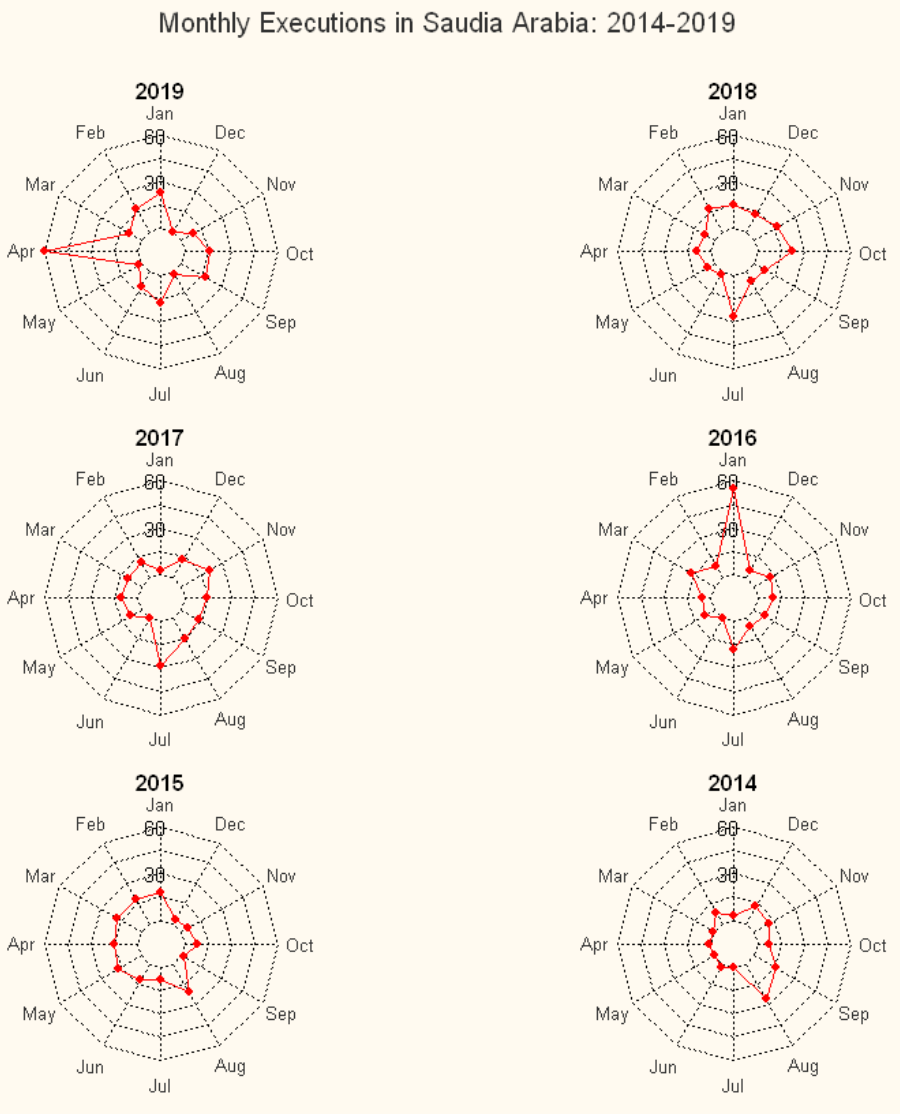
The axes here range from 0 to 60, and we see a couple of discrete spikes of 60 executions in April 2019 and January 2016. These spikes correspond to mass executions of dozens of alleged terrorism offenders at those time, though in reality many of those individuals were innocent religious minorities, peaceful protestors, and children.
The code for this viz looks like this:
library(fmsb)

[//]: # Reading in the data from .csv file. This .csv contains approximately 700 rows, each of which contains information on a discrete individual executed in Saudi Arabia between 2014 and 2019
KSA <- read.csv ("KSA_individuals_csv.csv", header=TRUE, sep=",")

[//]: # Converting date of execution column to date type
KSA$Date.of.execution <- as.Date (KSA$Date.of.execution, "%m/%d/%Y")

[//]: # Creating execution month and year columns
KSA$Execution.month <- format(KSA$Date.of.execution, "%m")
KSA$Execution.year <- format(KSA$Date.of.execution, "%Y")

[//]: # Converting month and year columns to numeric so the for loop below doesn't exclude months 01-09
KSA$Execution.month <- as.numeric(KSA$Execution.month)
KSA$Execution.year <- as.numeric(KSA$Execution.year)

[//]: # Creating five empty lists of 12 NULL values, to be filled by the for loop
ksa_years_list_2014 <- vector("list", 12)
ksa_years_list_2015 <- vector("list", 12)
ksa_years_list_2016 <- vector("list", 12)
ksa_years_list_2017 <- vector("list", 12)
ksa_years_list_2018 <- vector("list", 12)
ksa_years_list_2019 <- vector("list", 12)


[//]: # for loop that fills each slot of the empty lists with the length of the execution month column (i.e. number of executions) for each month
for (i in 1:12) {
    ksa_years_list_2014[[i]] <- length((subset(KSA,
        KSA$Execution.month == i & KSA$Execution.year == 2014))$Execution.month)

    ksa_years_list_2015[[i]] <- length((subset(KSA,
        KSA$Execution.month == i & KSA$Execution.year == 2015))$Execution.month)

    ksa_years_list_2016[[i]] <- length((subset(KSA,
        KSA$Execution.month == i & KSA$Execution.year == 2016))$Execution.month)

    ksa_years_list_2017[[i]] <- length((subset(KSA,
        KSA$Execution.month == i & KSA$Execution.year == 2017))$Execution.month)

    ksa_years_list_2018[[i]] <- length((subset(KSA,
        KSA$Execution.month == i & KSA$Execution.year == 2018))$Execution.month)

    ksa_years_list_2019[[i]] <- length((subset(KSA,
        KSA$Execution.month == i & KSA$Execution.year == 2019))$Execution.month)
}

[//]: # Turning each list into a dataframe
ksa_2014_ex <- data.frame(ksa_years_list_2014)
ksa_2015_ex <- data.frame(ksa_years_list_2015)
ksa_2016_ex <- data.frame(ksa_years_list_2016)
ksa_2017_ex <- data.frame(ksa_years_list_2017)
ksa_2018_ex <- data.frame(ksa_years_list_2018)
ksa_2019_ex <- data.frame(ksa_years_list_2019)


[//]: # Renaming the dataframe columns
colnames (ksa_2014_ex) <- c ("Jan", "Feb", "Mar", "Apr", "May", "Jun", "Jul", "Aug", "Sep", "Oct", "Nov", "Dec")
colnames (ksa_2015_ex) <- c ("Jan", "Feb", "Mar", "Apr", "May", "Jun", "Jul", "Aug", "Sep", "Oct", "Nov", "Dec")
colnames (ksa_2016_ex) <- c ("Jan", "Feb", "Mar", "Apr", "May", "Jun", "Jul", "Aug", "Sep", "Oct", "Nov", "Dec")
colnames (ksa_2017_ex) <- c ("Jan", "Feb", "Mar", "Apr", "May", "Jun", "Jul", "Aug", "Sep", "Oct", "Nov", "Dec")
colnames (ksa_2018_ex) <- c ("Jan", "Feb", "Mar", "Apr", "May", "Jun", "Jul", "Aug", "Sep", "Oct", "Nov", "Dec")
colnames (ksa_2019_ex) <- c ("Jan", "Feb", "Mar", "Apr", "May", "Jun", "Jul", "Aug", "Sep", "Oct", "Nov", "Dec")

[//]: # Combining all the dataframe rows into one dataframe
ksa_final <- rbind(ksa_2014_ex, ksa_2015_ex, ksa_2016_ex, ksa_2017_ex, ksa_2018_ex, ksa_2019_ex)

[//]: # Renaming the new dataframe rows
rownames (ksa_final) <- c(2014, 2015, 2016, 2017, 2018, 2019)

[//]: # To use radarchart(), the df has to have max and min values in each column. The below adds max and min rows of 0 and 60, each repeating 12 times
ksa_final <- rbind(ksa_final, (rep.int(60, 12)))
ksa_final <- rbind(ksa_final, (rep.int(0, 12)))

[//]: # Rearranging the rows because the pattern of rows for radarchart() to work has to be max, min, data:
ksa_final <- ksa_final[c(7,8,6,5,4,3,2,1),]


[//]: # Making the chart matrix
par(mar=c(1, 1, 1, 1), #decrease default margin
   oma=c(0,0,5,0),
   bg = "floralwhite",
   cex = 1,
   col="gray20"
   )
layout(matrix(1:6, ncol=2))
radarchart(ksa_final[c(1,2,3),],
           title = 2019,
          axistype=1,
           caxislabels=c("","",30,"",60),
          calcex=1.1,
          axislabcol="black",
           cglcol="black",
           pcol=2)
radarchart(ksa_final[c(1,2,5),],
           title = 2017,
           axistype=1,
           caxislabels=c("","",30,"",60),
          calcex=1.1,
          axislabcol="black",
           cglcol="black",
           pcol=2)
radarchart(ksa_final[c(1,2,7),],
           title = 2015,
           axistype=1,
           caxislabels=c("","",30,"",60),
          calcex=1.1,
          axislabcol="black",
           cglcol="black",
           pcol=2)
radarchart(ksa_final[c(1,2,4),],
           title = 2018,
           axistype=1,
           caxislabels=c("","",30,"",60),
          calcex=1.1,
          axislabcol="black",
           cglcol="black",
           pcol=2)
radarchart(ksa_final[c(1,2,6),],
           title = 2016,
           axistype=1,
           caxislabels=c("","",30,"",60),
          calcex=1.1,
          axislabcol="black",
           cglcol="black",
           pcol=2)
radarchart(ksa_final[c(1,2,8),],
           title = 2014,
           axistype=1,
           caxislabels=c("","",30,"",60),
          calcex=1.1,
          axislabcol="black",
           cglcol="black",
           pcol=2)
mtext("Monthly Executions in Saudia Arabia: 2014-2019", side = 3, line = 2, outer = TRUE)
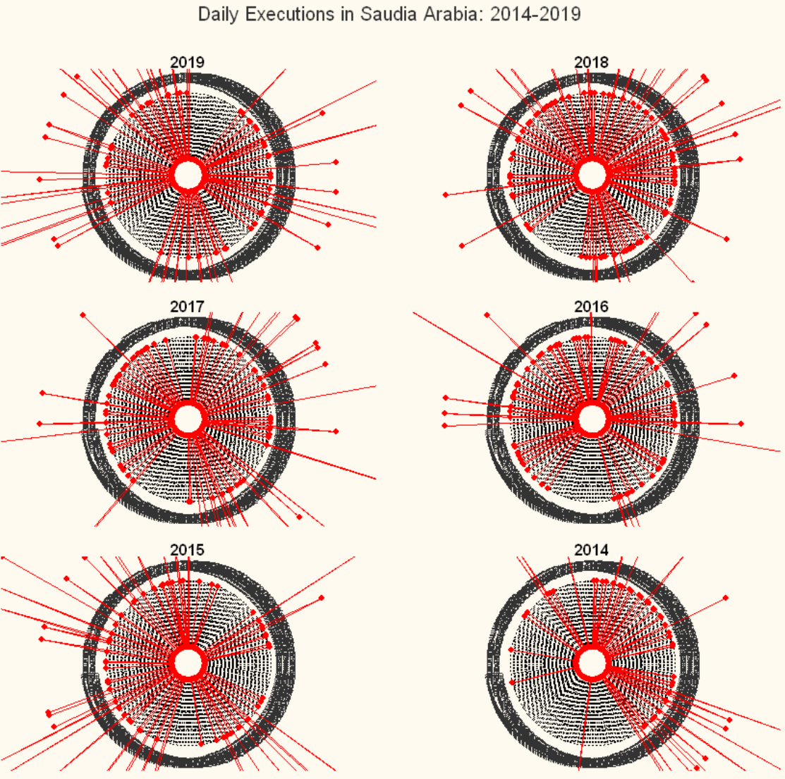
Radar charts of executions in Saudi Arabia by day
Finally, I plotted daily executions in Saudi Arabia by day. As with the Egypt example, the outer limit of the axes on these charts is 1, so the charts show you which periods of which years had zero executions, which had one execution, and which had more than one execution. As such, we can see the extent to which death sentences were evenly distributed throughout a given year, and where there were gaps.
The code for this viz looks like this:
library(fmsb)

[//]: # Reading in the data from .csv file. This .csv contains approximately 700 rows, each of which contains information on a discrete individual executed in Saudi Arabia between 2014 and 2019
KSA <- read.csv ("KSA_individuals_csv.csv", header=TRUE, sep=",")

[//]: # Converting date of execution column to date type
KSA$Date.of.execution <- as.Date (KSA$Date.of.execution, "%m/%d/%Y")

[//]: # Creating Execution.day.of.year and Execution.year columns
KSA$Execution.day.of.year <- format(KSA$Date.of.execution, "%j")
KSA$Execution.year <- format(KSA$Date.of.execution, "%Y")

[//]: # Converting Execution.day.of.year and Execution.year to numeric:
KSA$Execution.day.of.year <- as.numeric(KSA$Execution.day.of.year)
KSA$Execution.year <- as.numeric(KSA$Execution.year)

[//]: # Creating empty lists of 365 NULL Values
ksa_daily_2014_list <- vector("list", 365)
ksa_daily_2015_list <- vector("list", 365)
ksa_daily_2016_list <- vector("list", 365)
ksa_daily_2017_list <- vector("list", 365)
ksa_daily_2018_list <- vector("list", 365)
ksa_daily_2019_list <- vector("list", 365)

[//]: # for loop that fills each slot of the empty lists with the length of the Execution.month column (i.e. number of executions) for each month
for (i in 1:365) {
    ksa_daily_2014_list[[i]] <- length((subset(KSA,
        KSA$Execution.day.of.year == i & KSA$Execution.year == 2014))$Execution.day.of.year)

    ksa_daily_2015_list[[i]] <- length((subset(KSA,
        KSA$Execution.day.of.year == i & KSA$Execution.year == 2015))$Execution.day.of.year)

    ksa_daily_2016_list[[i]] <- length((subset(KSA,
        KSA$Execution.day.of.year == i & KSA$Execution.year == 2016))$Execution.day.of.year)

    ksa_daily_2017_list[[i]] <- length((subset(KSA,
        KSA$Execution.day.of.year == i & KSA$Execution.year == 2017))$Execution.day.of.year)

    ksa_daily_2018_list[[i]] <- length((subset(KSA,
        KSA$Execution.day.of.year == i & KSA$Execution.year == 2018))$Execution.day.of.year)

    ksa_daily_2019_list[[i]] <- length((subset(KSA,
        KSA$Execution.day.of.year == i & KSA$Execution.year == 2019))$Execution.day.of.year)

    }

[//]: # Turning each list into a dataframe
ksa_2014_daily_df <- data.frame(ksa_daily_2014_list)
ksa_2015_daily_df <- data.frame(ksa_daily_2015_list)
ksa_2016_daily_df <- data.frame(ksa_daily_2016_list)
ksa_2017_daily_df <- data.frame(ksa_daily_2017_list)
ksa_2018_daily_df <- data.frame(ksa_daily_2018_list)
ksa_2019_daily_df <- data.frame(ksa_daily_2019_list)


[//]: # Renaming the dataframe columns
colnames (ksa_2014_daily_df) <- c(1:365)
colnames (ksa_2015_daily_df) <- c (1:365)
colnames (ksa_2016_daily_df) <- c (1:365)
colnames (ksa_2017_daily_df) <- c (1:365)
colnames (ksa_2018_daily_df) <- c (1:365)
colnames (ksa_2019_daily_df) <- c (1:365)

[//]: # Combining all the dataframe rows into one dataframe
ksa_daily_final <- rbind(ksa_2014_daily_df, ksa_2015_daily_df, ksa_2016_daily_df, ksa_2017_daily_df, ksa_2018_daily_df, ksa_2019_daily_df)

[//]: # Renaming the new dataframe rows
rownames (ksa_daily_final) <- c(2014, 2015, 2016, 2017, 2018, 2019)

[//]: # To use radarchart(), the df has to have max and min values in each column. The below adds max and min rows of 0
# and 1, each repeating 365 times
ksa_daily_final <- rbind(ksa_daily_final, (rep.int(1, 365)))
ksa_daily_final <- rbind(ksa_daily_final, (rep.int(0, 365)))

[//]: # Rearranging the rows because the pattern of rows for radarchart() to work has to be max, min, data:
ksa_daily_final <- ksa_daily_final[c(7,8,6,5,4,3,2,1),]

[//]: # Making the chart matrix
par(mar=c(1, 1, 1, 1), #decrease default margin
   oma=c(0,0,5,0),
   bg = "floralwhite",
   cex = 1,
   col="gray20"
   )
layout(matrix(1:6, ncol=2))
radarchart(ksa_daily_final[c(1,2,3),],
           title = 2019,
          axistype=1,
           caxislabels=c("","","","",""),
          calcex=1.1,
          axislabcol="darkgreen",
           cglcol="black",
           pcol=2)
radarchart(ksa_daily_final[c(1,2,5),],
           title = 2017,
           axistype=1,
           caxislabels=c("","","","",""),
          calcex=1.1,
          axislabcol="darkgreen",
           cglcol="black",
           pcol=2)
radarchart(ksa_daily_final[c(1,2,7),],
           title = 2015,
           axistype=1,
           caxislabels=c("","","","",""),
          calcex=1.1,
          axislabcol="darkgreen",
           cglcol="black",
           pcol=2)
radarchart(ksa_daily_final[c(1,2,4),],
           title = 2018,
           axistype=1,
           caxislabels=c("","","","",""),
          calcex=1.1,
          axislabcol="darkgreen",
           cglcol="black",
           pcol=2)
radarchart(ksa_daily_final[c(1,2,6),],
           title = 2016,
           axistype=1,
           caxislabels=c("","","","",""),
          calcex=1.1,
          axislabcol="darkgreen",
           cglcol="black",
           pcol=2)
radarchart(ksa_daily_final[c(1,2,8),],
           title = 2014,
           axistype=1,
           caxislabels=c("","","","",""),
          calcex=1.1,
          axislabcol="darkgreen",
           cglcol="black",
           pcol=2)
mtext("Daily Executions in Saudia Arabia: 2014-2019", side = 3, line = 2, outer = TRUE)