Building and bootstrapping logistic regression models to predict executions in Egypt

As discussed elsewhere in this portfolio, my prior human rights work with Reprieve involved the creation of the Egypt Death Penalty Index (EDPI), a comprehensive database tracking all known capital trials in Egypt since 2013, and many from before then as well. The resulting data provides an important real-time view into the Egyptian government’s application of capital punishment. The database allows human rights defenders to examine ongoing capital trials and identify individuals in need of legal assistance, which is largely how the EDPI has been used to date.

But given that the EDPI contains such rich historical information on hundreds of capital trials, I wondered if this information could also serve as the basis for machine learning modeling to predict the outcomes of future capital trials based on their characteristics. Specifically, I wondered if I could build models that would identify which factors related to a capital trial might increase the likelihood that a defendant would go on to be executed. In the EDPI dataset, each row represents one individual who received a prelmiinary death sentence in an Egyptian court. The dataset contains dozens of columns containing demographic and legal information about each individual, including age, gender, location of arrest, alleged offence, and details about what happened at each stage of the legal process in the individuals trial(s). Crucially, the dataset also indicates whether each individual indeed went on to be executed, or if some other outcome occured (acquittal, commutation, etc.). This is an ideal structure for classification modeling to predict how likely future individuals are to be executed, based on demographic and legal information. The project below represents my attempt to use logistic regression to answer this question.

Paring down raw data

The first step was to pare down the raw data that forms the back end of the EDPI (downloadable here) into a format that could serve as the basis for modeling. The EDPI data contains a wealth of information about individual defendants, all of which has important uses, but not all of it is useful for the purposes of predictive modeling. For this project, I used my domain expertise to narrow the data down to the variables I thought most relevant:

• Whether or not an individual was ultimately executed (column name executed_0_1). This is be the response variable. Any individual who was ultimately executed received a 1 in this column, anyone who was not executed received a 0.
• Whether the offence was “political” or “criminal” in nature–that is, whether the alleged facts of the case and the perceived motivation for the commission of the offence were in some way connected to the political and societal changes that have arisen in Egypt since the January 2011 revolution or not (column name category_of_offence).
• The gender of the defendant (column name defendant_gender).
• Whether the defendant was tried in a civilian court or a military tribunal (column name court_type).
• Whether the defendant was tried in absentia or was present during proceedings (column name defendant_status).
• The amount of time elapsed between the defendant’s alleged offence and the court reaching a verdict in that defendant’s case in the first instance (column name days_btwn_offence_and_crim_1_judgement).
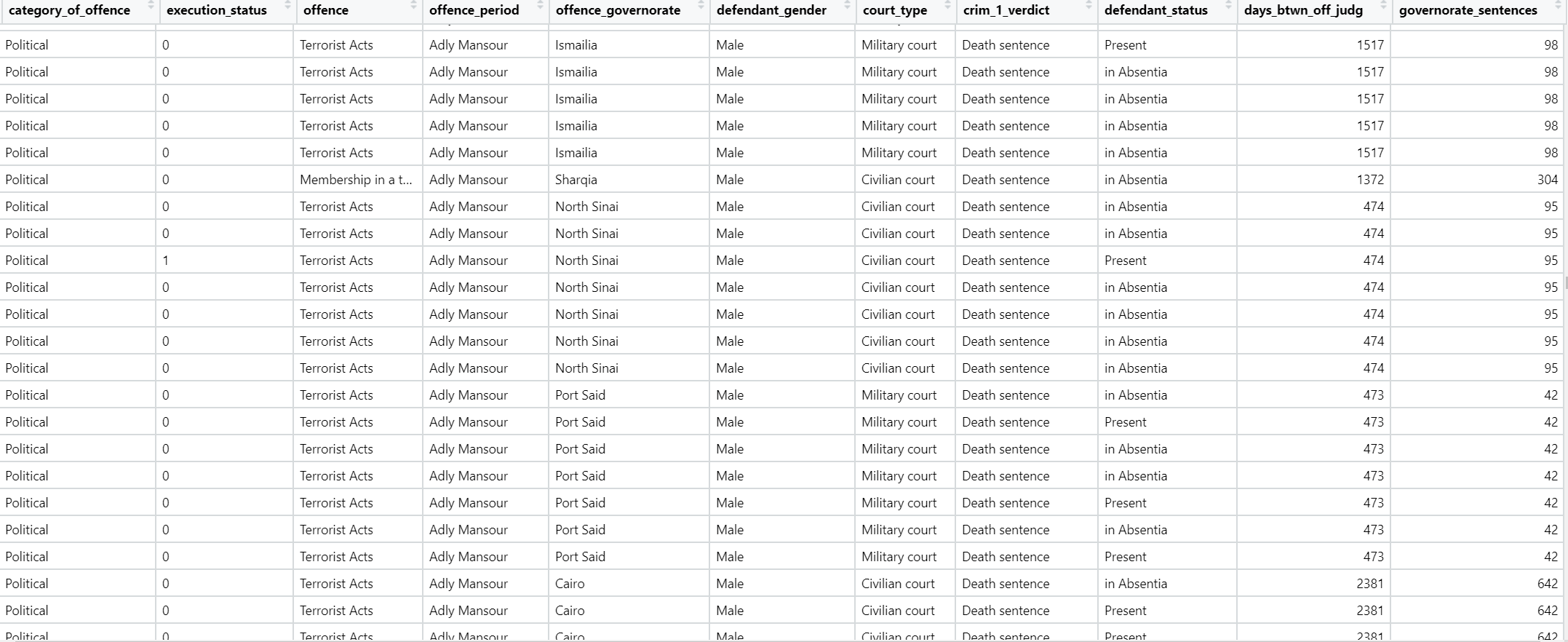
• The number of overall death sentences handed down in the governorate where the individual in question was being tried (column name governorate_sentences).

The final dataset looked like this:

Building and bootstrapping a logit model

I started by omitting NA values from the data (necessary for the bootstrapping process used below). Then I split the data into training and test sets, with a 70/30 split. I used the sample.split() function from the caTools library, as this function preserves the relative ratio of zeroes and ones in the response column, ensuring that our training and test sets resemble each other:

library(caTools)

EDPI <- na.omit(EDPI)

split = sample.split(EDPI$execution_status, SplitRatio = 0.70)
EDPI_train = subset(EDPI, split==TRUE)
EDPI_test = subset(EDPI, split==FALSE)

Next, I built the logistic regression model using the glm() package:

library(glmnet)

boot_log_model <- glm(execution_status ~ + category_of_offence + governorate_sentences + court_type +
                      defendant_gender + days_btwn_offence_and_crim_1_judgement,
                      data = EDPI2, family = binomial (link = 'logit'))

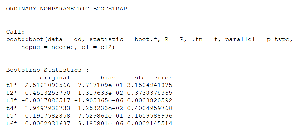
Then, I fed the logit model to the Boot() function from the car library and specified 2000 bootstrapping samples:

library(car)

results <- Boot(boot_log_model, f = coef, R = 2000)

Finally, I pulled out relevant information about the final boostrapped model, including coefficients and p-values:

Names = names(results$t0)
SEs = sapply(data.frame(results$t), sd)
Coefs = as.numeric(results$t0)
zVals = Coefs / SEs
Pvals = 2*pnorm(-abs(zVals))
Significant = ifelse(Pvals <= .001, "***", ifelse(Pvals > .001 & Pvals <= .01, "**", ifelse(Pvals > .01 & Pvals <= .05, "*",
                                                                             ifelse(Pvals >.05 & Pvals <= .1, ".",
                                                                                   " "))))

Formatted_Results = cbind(Names, Coefs, SEs, zVals, Pvals, Significant)
Formatted_Results

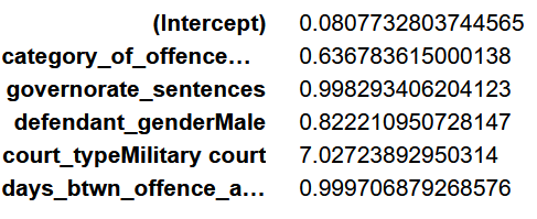
The results looked like this:

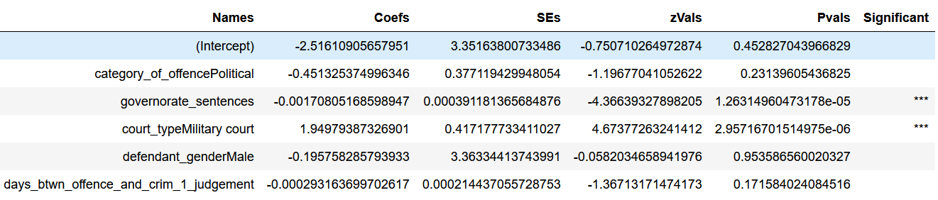
From this, we see that the model has identified two significant variables correlated with executions: the number of death sentences previously handed down in the governorate where the death sentence in question occurred (“governorate_sentences”) and trials that took place in a military court (“court_typeMilitary court”). Interpretations of these results are provided in the following section. First, I wanted to check the bootstrapped AUC and accuracy. To do that, I wrote a function that extracts the bootstrapped AUC for all 2000 samples and calculates the optimism (difference between in-sample and bootstrapped AUC) for each sample. We can then take the average optimism and subtract it from the overall in-sample /original AUC to obtain the overall bootstrapped AUC. As below, bootstrapped AUC for this model was .8011. (Non-bootstrapped AUC was only slightly higher, at .8013, eliminating worries about overfitting):

library(ROCR)

R = 2000
n = nrow(EDPI2)

# Build empty Rx2 matrix for bootstrap results 
B = matrix(nrow = R, ncol = 2,
           dimnames = list(paste('Sample',1:R),
                           c("auc_orig","auc_boot")))

for(i in 1:R){
    
[//]: # draw a random sample
    obs.boot <- sample(x = 1:n, size = n, replace = T)
    data.boot <- EDPI2[obs.boot, ]
    
[//]: # fit the model on bootstrap sample
    boot_log_model <- glm(execution_status ~ + category_of_offence + governorate_sentences
            + defendant_gender + court_type +
            days_btwn_offence_and_crim_1_judgement, data = EDPI2, family = binomial (link = 'logit'))
    
[//]: # apply model to original data
    prob1 = predict(boot_log_model, EDPI2, type='response')

[//]: # Note that prediction() in ROCR has problems sometimes because there are other libraries with functions called prediction(), so make sure to write it as ROCR:prediction(). See here for more: https://stackoverflow.com/questions/39483744/rocr-library-prediction-function-error
    pred1 = ROCR::prediction(prob1, EDPI2$execution_status)
    auc1 = performance(pred1,"auc")@y.values[[1]][1]
    B[i, 1] = auc1
    
[//]: # apply model to bootstrap data
    prob2 = predict(boot_log_model, data.boot, type='response')
[//]: # Note that prediction() in ROCR has problems sometimes because there are other libraries with functions called prediction(), so make sure to write it as ROCR:prediction(). See here for more:
[//]: # https://stackoverflow.com/questions/39483744/rocr-library-prediction-function-error
    pred2 = ROCR::prediction(prob2, data.boot$execution_status)
    auc2 = performance(pred2,"auc")@y.values[[1]][1]
    B[i, 2] = auc2
}

[//]: # Turn B into data frame
B <- as.data.frame(B)

[//]: # Create optimism column
B$optimism <- B$auc_boot - B$auc_orig

in_sample_auc <- mean(B$auc_orig)
avg_AUC_bootstrap <- mean(B$auc_boot)
avg_optimism <- mean(B$optimism)

bootstrapped_auc = in_sample_auc - avg_optimism
bootstrapped_auc

Finally, I wanted to check for multicollinearity, to ensure that my model did not have correlated predictor variables.

library(car)
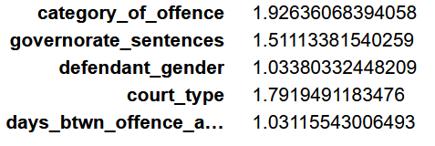
vif(boot_log_model)

Generally, Variance Inflation Factor (VIF) values below 5 generally indicate no multicollinearity, so it does not appear to be a problem here:

Interpreting results and accuracy

As above, the two significant variables here were the number of death sentences previously handed down in the governorate where the death sentence in question occurred (“governorate_sentences”) and trials that took place in a military court (“court_typeMilitary court”). If we exponentiate the coefficients for those variables, we get the following:

exp(coef(boot_log_model))

Based on the above, we could conclude:

• Controlling for other variables, the odds of eventual execution were 6.02 times (602%) higher for individuals convicted in a military tribunal, as opposed to a civilian court.
• Controlling for other variables, the odds that an individual would go on to be executed were reduced by .002 times (0.2%) for every additional death sentence handed down in the governorate where the defendant in question was sentenced to death.

Intuitively, this makes sense. It has long been known that people sentenced to death in military trials in Egypt are especially at risk of being executed. It also tracks that people sentenced to death in governorates that have previously handed down large numbers of death sentences are less likely to be executed–many of the governorates where the most death sentences have been issued have received considerable negative international media attention, which tends to decrease the likelihood that executions are carried out.

Based on the significant variables, the intuitive interpretation of those variables, and the high bootstrapped AUC, this seems like a useful model. One important thing to check, however, is how this model’s accuracy compares to the accuracy of a naive baseline model. To find this, we first calculate the accuracy of our current model. Based on popular convention, we will do this with a 50% probability threshold, meaning that if the model predicts that an individual had a more than 50% probability of execution, that will be counted as a “yes”, and less than 50% probability of execution will be counted as a “no”:

boot_log_probs <- predict(boot_log_model, type = "response", newdata = EDPI2)
tbl <- table(boot_log_probs > 0.5, EDPI2$execution_status)
accuracy = sum(diag(tbl))/sum(tbl)

The accuracy here is 97.57%, which is suspiciously high, given that AUC was only about 0.80. This suggests there are significant type I or type II errors–more on that in a minute. First, we will check the accuracy of the naive baseline model. To do that, we first find which class, 0 or 1, is more common in our response column. We find that there are more zeroes, so our naive baseline model will be to predict 0 (i.e. “not executed”) for every case. We then take the number of zeroes in the data and divide it by the number of rows in the data to obtain our baseline model accuracy:

nrow(subset(EDPI2, EDPI2$execution_status == 1))
nrow(subset(EDPI2, EDPI2$execution_status == 0))
nrow(subset(EDPI2, EDPI2$execution_status == 0))/nrow(EDPI2)

Here, we see that our baseline model accuracy is … 97.57%. This is exactly the same as our logit model, meaning that our logistic regression model is exactly as accurate as the baseline model. If we investigate further, we can see the reason for this:

tbl <- table(boot_log_probs > 0.5, EDPI2$execution_status)
tbl

If we run the above code, we see the culprit: using a 50% probability threshold, our model predicted that every individual in the dataset would not be executed, which is the same as our baseline model. At first glance, this might seem bad; if our logistic regression model is only as accurate as a naive baseline, is it even useful? But actually, yes, the logistic regression model is still quite useful, for a couple of reasons.

First, we should note that 50% is a very arbitrary probability threshold when it comes to predicting something like whether an individual will be executed. There is no reason why a predicted probability of execution in excess of 50% should mean that someone “will” be executed, and a probability of less than 50% means that they will not. For example, if the model predicted than individual had a 40% likelihood of execution, that would still be cause for concern. And indeed, if we reduce our probability threshold, the model predicts many more executions.

Second, the logistic regression model provides us with several pieces of important information that the baseline model does not. One such piece of information is the ranked probabilities of execution for every individual in the dataset:

execution_probabilities <- predict(boot_log_model, EDPI2, type = "response") 
sort(execution_probabilities, decreasing = TRUE)

We can append these probabilities to our original dataset and identify which individuals are at greatest risk of execution, which is a hugely useful piece of information. Additionally, we also know which variables are significantly correlated with increased likelihood of execution, which is important information, even as a heuristic device.

Use cases

I envision a number of important use cases for this kind of modeling. Imagine a human rights NGO that works to assist people facing death sentences in Egypt: with thousands of individuals sentenced to death in Egypt in recent years, it is difficult for human rights groups to know where to invest their limited resources. A sorted list of the individuals who are most likely to be executed would be a powerful tool for such organizations to use in prioritizing resource allocation. Coalitions of NGOs and political allies must also make similar decisions when deciding where to deploy trial monitoring resources.

More broadly, having a sound statistical understanding of which factors are most correlated with executions is important from a qualitative standpoint, as it helps to indicate which issue areas require greater attention from human rights advocates and policymakers. For example, the findings of this modeling could certainly serve as the basis for a narrative report from a human rights organization focused on the dangers of Egypt’s military court system. I really believe that these are crucial applications of data science that need to be more widely implemented in the human rights investigations field.